ParSA Results

Solutions

Interferograms

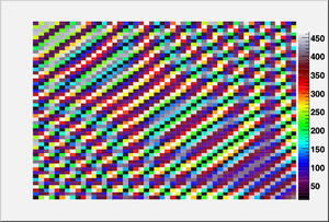
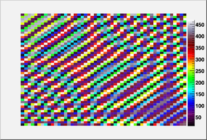
The set of images in Fig. 1 and Fig. 2 depict the test interferogram analyzed using ParSA and the best interferogram solution found by ParSA. When compared visually, the two interferograms are nearly indistinguishable. This comparison shows that the solution found by the ParSA algorithm is a good one.

Figure 1: The test interferogram created from three random surfaces.

Figure 2: The best solution found amongst several simulated annealing runs.

Surfaces

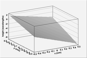
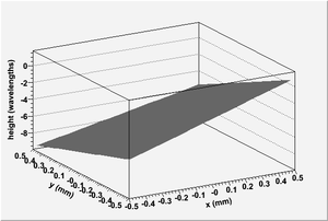
Fig. 3 and Fig. 5 show the front and back surfaces of the diamond wafer used to create the test interferogram depicted in Fig. 1. Fig. 4 and Fig. 6 show the solutions found by the ParSA algorithm which generated the interferogram shown in Fig. 2. The incident light used to create each of the interferograms is incident in the z-direction. The test diamond surfaces are the same shape and are apparently planar, with the exception that they have a small contribution from a second order Legendre polynomial . This slight curvature can be seen in the complex dark and light band structure depicted in Fig. 1. If the surfaces were actually planar as they appear, the resulting interferogram would not have these rich features and would simply be a series of straight, equally-spaced, light and dark bands.

Figure 3: The front diamond surface used to generate the interferogram in the test problem.

Figure 4: The best solution found amongst several simulated annealing runs.

The solutions found by simulated annealing feature two ambiguities that are a result of the nature of light. The first ambiguity results from the fact that a mirror transformation of the surfaces about a vertical plane do not change the interferogram. The second ambiguity is a result of the periodic nature of light and can be seen in differences present in the distances between surfaces between the test and solution surfaces.

Figure 5: The back diamond surface used to generate the interferogram in the test problem.

Figure 6: The best solution found amongst several simulated annealing runs.

Performance

MIR Performance

The ParSA library documentation gives the following equation which can be used to estimate performance of an MIR run

$P(\chi _{n}\notin Cost_{min})\sim \left({\frac {K}{n}}\right)^{\alpha }$

where P is the probability of non-convergence, $\chi _{n}$ is a solution of a run of length n, $Cost_{min}$ is the minimum acceptable solution, and K and $\alpha$ are problem specific parameters. K and $\alpha$ can be determined by plotting the Bayesian estimator for P versus n on a log scale and determining the slope and y-intercept. The expression for the Bayesian estimator ${\hat {p}}$ is given by

${\hat {p}}={\frac {n_{f}+1}{N+2}}$

where $n_{f}$ is the number of runs whos cost function value is greater than $Cost_{min}$ and N is the total number of runs.

Figure 7: Log of probability versus non-convergence versus log of run length for alpha=0.5.

Figure 8: Log of probability versus non-convergence versus log of run length for alpha=0.9.

alpha = 0.5

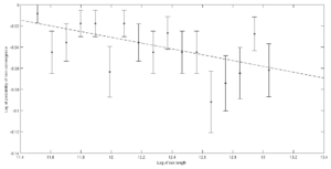
Fig. 7 shows the log plot of probability of non-convergence versus run length for a MIR run with the alpha cooling parameter set to 0.5. The slope and y-intercept of the linear least-squares fit are $-0.0273\pm 0.0103$ and $0.297\pm 0.127$ with a reduced $\chi ^{2}$ value of 1.0. K and $\alpha$ were then determined to be $(5.31\pm 2.4)\times 10^{4}$ and $0.0273\pm 0.0103$.

alpha = 0.9

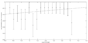
Fig. 8 shows the log plot for a MIR run with the cooling parameter alpha set to 0.9. The slope and y-intercept of the linear least-squares fit are $0.0047\pm 0.0060$ and $-0.070\pm 0.074$ with a reduced $\chi ^{2}$ value of 0.55. K and $\alpha$ were then determined to be $(0.03\pm 1.2)\times 10^{8}$ and $-0.0047\pm 0.0060$. Runs of greater lengths will be needed to determine these parameters for this value of alpha.